Let’s take the natural numbers (without zero) and order them under the division relation. So we completely forget the usual inequality \(\leq\) between natural numbers, and we now say that \(a \leq b\) whenever \(a\) divides \(b\). So \(1\) is the smallest element and we have chains like \(1 \leq 2 \leq 4 \leq 16 \leq \dots\). The result is called the big cell (a terminology first used by John Horton Conway). How can we best visualize this big cell? Let’s make some animated GIFs.
Lieven Le Bruyn proved in “Covers of the Arithmetic Site” (Theorem 1) that the big cell is a Diaconescu cover for the Arithmetic Site by Connes and Consani. The topological space corresponding to the big cell is the space \(\mathbb{S}\) of supernatural numbers, with the localic topology. The problem is that this topology is not Hausdorff. So for intuition and visualization, it makes more sense to look at the patch topology, generated by the compact opens for the original topology and their complements. By replacing the original topology with the patch topology, we now get a compact metric space.
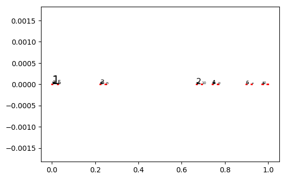
In fact, we can see the supernatural numbers with the patch topology as a closed subset of the Cantor set, but this “visualization” is not very insightful:
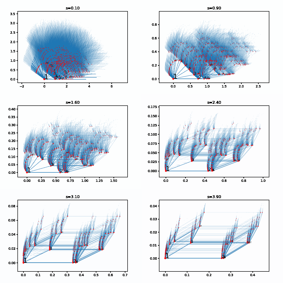
So we take a different approach: each prime number will be plotted in a different angle relative to the origin, and the powers \(1,p,p^2,p^3,\dots\) of a fixed prime \(p\) will be drawn on a line. As distance between \(1\) and \(p^k\) we take \(\sqrt{\sum_{i=1}^k p^{-is}}\), where \(s\) is a free parameter. To make sure that the induced topology is the patch topology, we have to take \(s > 2\).
The result depends on the way that you pick the angles for each prime number. Here is a first possibility, using an arctangent function.
And here another one where the angles “follow a Bell curve”.
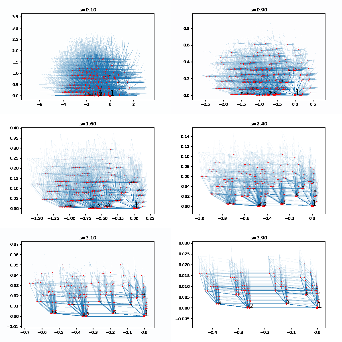
The topological space that we are interested in, is the space consisting of the red dots. The blue lines show the divisibility relation.
As formula for the distance between \(1\) and \(p^k\) I originally used \(\sum_{i=1}^k p^{-is}\), without the square root. This comes closer to how I wrote it down in my thesis, but the GIFs are less interesting… here are some of them:
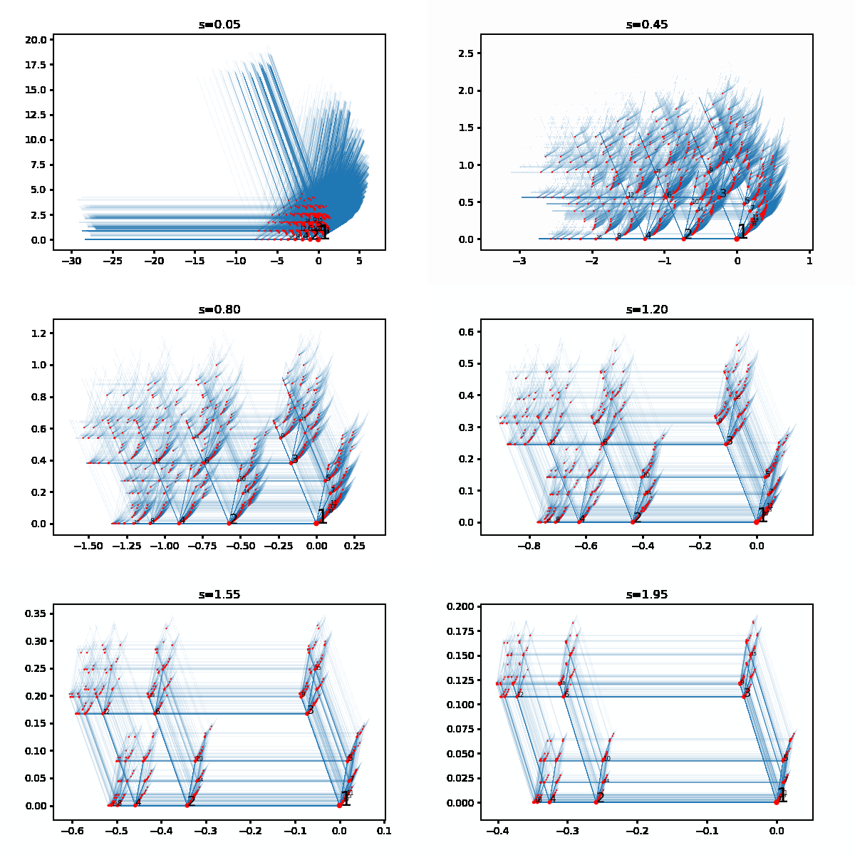
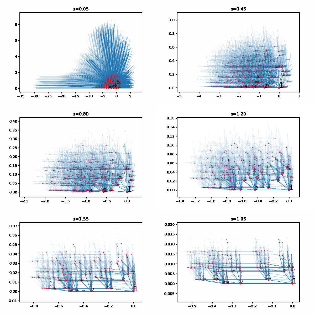
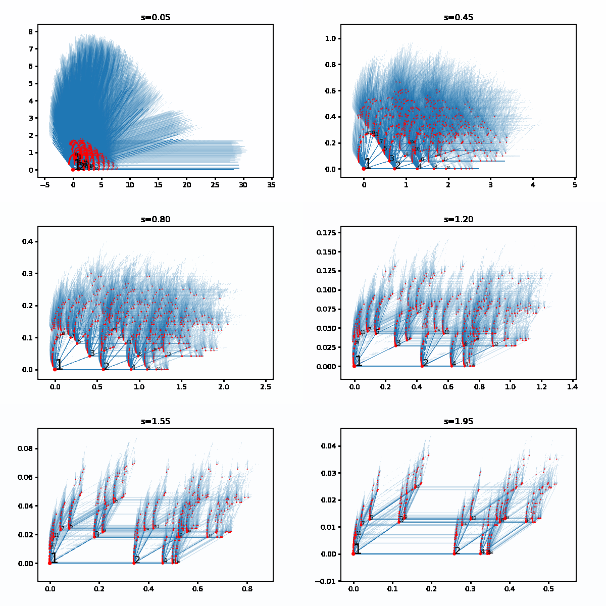
And here is the Python code that I used. Make sure to edit the last line with the location where you want to save the GIF. I execute the code as two cells in a Jupyter notebook, and for me it takes 1 or 2 minutes to generate one of the GIFs. For the animations above, the choices for (f,g) are (f3,g2), (f2,g2), (f1,g1), (f2,g1) and (f3,g1), in this order.
from primefac import factorint,primes
from math import cos,sin,log,pi,e,sqrt,exp,atan

# Lower is better but slower.
precision = 0.01

# Only consider prime numbers < prime_bound.
# Larger primes would be plotted close to the origin anyway.
prime_bound = 100
prime_list = primes(prime_bound)

# Only plot integers < integer_bound.
integer_bound = 1000

# Functions converting a prime number to an angle.
# For each prime, it gives an angle in radians
# with respect to the origin.
# Plot makes more sense if difference between two angles
# is at most pi.
def f1(n):
    return log(2.0)/log(n)*pi
def f2(n):
    x = (n-2)*0.1
    b = -0.5*pow(x,2)
    return exp(b)*pi
def f3(n):
    return 2*atan((n-2.0)/20)

# Pick one of the angle functions above.
f = f1

# Functions rescaling the lengths of the edges, default=g1.
# Only for aesthetic reasons.
# Note: together with s, this affects whether or not the result
# corresponds to a totally bounded subset of the real plane.

def g1(r):                      # result is bounded for s > 1
    return r
def g2(r):                      # result is bounded for s > 2
    return pow(r,0.5)
def g3(r):                      # result is bounded for s > .5
    return pow(r,2)

# Pick one of the rescaling functions above.
g = g1

# Adding two vectors.
def tuple_add(a,b):
    return tuple(item1 + item2 for item1, item2 in zip(a, b))

# Translating a line along a vector.
def translate(line,point):
    new_line = [ tuple_add(i,point) for i in line ]
    return new_line

# Length of the line going from 1 to p^k,
# before rescaling with g above.
def l(p,k,s):
    return pow(p,-s)*(1.0-pow(p,-k*s))/(1.0-pow(p,-s))

# Dictionary associating to each prime the corresponding angle.
alpha = { p:f(p) for p in prime_list }

# Location of p^infinity in the real plane.
# Rescaled using g above.
# Note: vertex(p^k,s) -> vertex_infinity(p,s) for k -> infinity.
def vertex_infinity(p,s):
    r = 1.0/(pow(p,s)-1.0)
    a = alpha[p]
    return (g(r)*cos(a),g(r)*sin(a))

# Dictionary associating to each prime p the line segment
# from 1 to p^infinity.
# For each n that is coprime with p, we can translate this line
# segment to get the line from n to n*p^infinity.
def rays(s):
    return { p:[(0,0),vertex_infinity(p,s)] for p in prime_list }

# Location of the natural number n in the real plane.
# Rescaled using g above.
# If n = p_1^e_1 * p_2^e_2 * ... * p_k^e_k, then
# vertex(n,s) is the sum of all the vertex(p_i^e_i,s)
# for i from 1 to k.
def vertex(n,s):
    v = (0,0)
    fac = factorint(n)
    for p,k in fac.items():
        if p < prime_bound:
            a = alpha[p]
            r = l(p,k,s)
            w = (g(r)*cos(a),g(r)*sin(a))
            v = tuple_add(v,w)
    return v

# For each n, add the rays from n to n*p^infinity,
# for all primes p coprime to n.
# Note: if p divides n, then we do not have to draw
# the ray from n to n*p^infinity, since it is already
# contained in the ray from m to m*p^infinity for some
# integer m coprime to p.
def add_rays(collection,n,s):
    v = vertex(n,s)
    for p in prime_list:
        if n % p != 0:
            r = rays(s)
            ray = r[p]
            collection.append(translate(ray,v))
    return collection
# Thanks to:
# https://stackoverflow.com/a/21357666                    (Plotting Line Segments)
# https://ndres.me/post/matplotlib-animated-gifs-easily       (Animated GIF)
%matplotlib inline
# Removing the line above breaks the code, for some reason.
import numpy as np
import matplotlib.pyplot as plt
from matplotlib import collections  as mc
import imageio

def big_cell(s):
    lines = []
    for n in range(1,integer_bound):                          # add rays flowing out of n
        lines = add_rays(lines,n,s)

    lines_array = np.array(lines)

    vertices = [vertex(n,s) for n in range(1,integer_bound)]  # coordinates of each integer n
    x = [ v[0] for v in vertices ]                            # x-coordinates
    y = [ v[1] for v in vertices ]                            # y-coordinates
    sizes = [20*pow(n,-0.6) for n in range(1,integer_bound)]  # size of the red dot for each n

    lc = mc.LineCollection(lines_array, linewidths=0.05)
    fig, ax = plt.subplots()
    ax.add_collection(lc)
    ax.scatter(x,y,c='red',s=sizes,zorder=10)                 # places the red dots on top
    for i in range(1,20):
        ax.annotate(str(i), (x[i-1], y[i-1]),color='black',size=20*pow(i,-0.5),zorder=11)
    ax.autoscale()
    ax.set(title="s="+('%.2f' % s))                           # display value of s

    fig.canvas.draw()       # draw the canvas, cache the renderer,
    image = np.frombuffer(fig.canvas.tostring_rgb(), dtype='uint8')
    image  = image.reshape(fig.canvas.get_width_height()[::-1] + (3,))
    plt.close('all')
    return image

kwargs_write = {'fps':1.0, 'quantizer':'nq'}

# Saves GIF to disk. Choose a file location, a duration of each frame, and the s-value for each frame.
imageio.mimsave('~/Desktop/bigcell.gif', [big_cell(0.05*i) for i in range(1,40)], duration=0.10)
